Homepage of Jörn Dinkla

Welcome to my homepage.
You can also find me on
GitHub
 ,
Slideshare
,
Slideshare
![]() and
YouTube
and
YouTube
![]() .
.
If you want to contact me, send me an email.
Generating dialogues with OpenAI's API
During the winter holidays I had some fun letting AIs discuss with each other about various topics. I personally like to chat with ChatGPT and challenge it (him/her) with difficult thoughts. I wondered if I can let ChatGPT argue with other instances of itself …
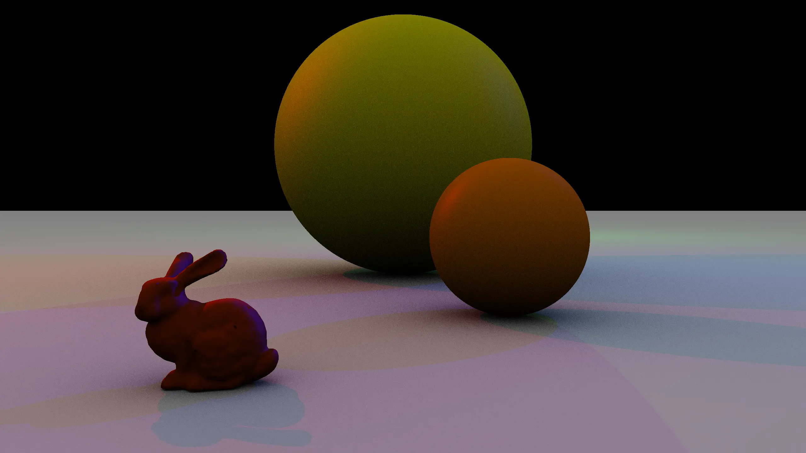
Using OpenAI's API to generate prompts for images
The advances of artificial intelligence in the last months are simply breath taking. It is now very easy to use “intelligent” APIs in your web app. In this example application the user can describe a scene in simple terms. GPT creates a fully fledged description and DALL-E 2 converts this into an image.


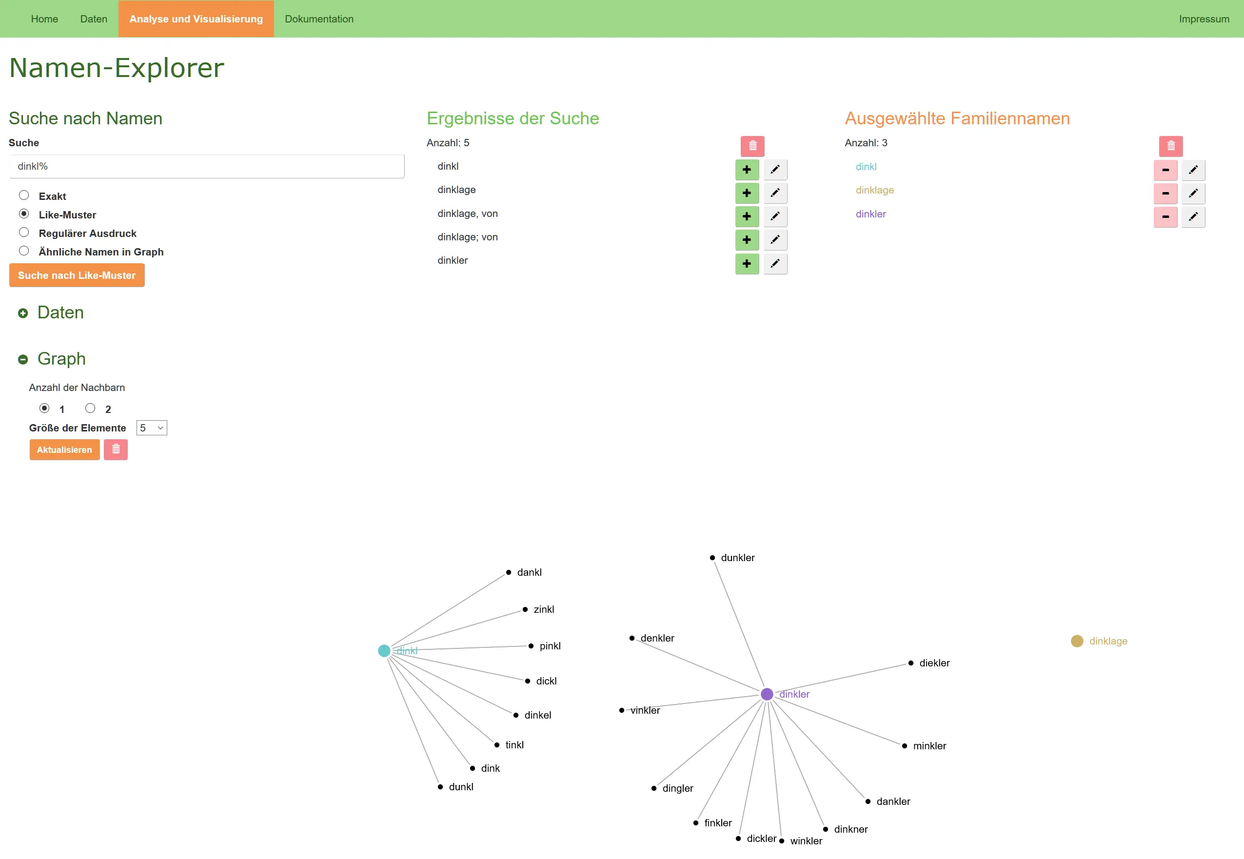


Groovy, EMF and UML2
I wrote the Groovy EMF builder and the Groovy UML2 builder.
These tools use the builder concept of the programming language Groovy to ease the processing of Eclipse Modelling Framework and UML2 code.
Eclipse BugDays 2007
I participated at Eclipse BugDays in July, August, September, October, and November 2007 and helped debugging the Eclipse projects JDT, PDE/UI, and ECF.
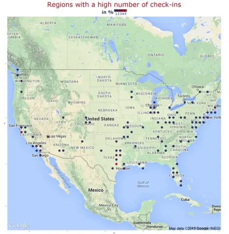
Fraud Detection with Artificial Intelligence
From 1999 to 2004, I collected information on the topic of ‘Fraud detection’ on my website.
When I started this in 1999 as a research assistant at the University of Karlsruhe, there was not much information available on the topic of ‘Data Science’. Back then, it was more commonly referred to as ‘Knowledge Discovery in Databases’ (KDD) in academic circles or ‘Data Mining’ in the business world.